A look back: emTeX

I first learned about document preparation programs when I entered university in 1990. At first, I wrote many of my class papers in DOS word processors like WordPerfect or Galaxy Write, but after I got an account on the Unix network, I started to explore other tools. I liked using nroff to write documents in plain text, which I could easily print to any campus printer.

As an undergraduate physics student, I needed to write reports for my lab classes. These reports usually needed to reference equations so I could discuss the experiment theory and then perform the analysis based on the equations of motion. Equations are not really something you can do in nroff. Then, a friend introduced me to LaTeX, and I immediately switched to that for writing my lab reports.

TeX, LaTeX, and emTeX

Don Knuth developed TeX so he could write his books, which included a lot of math and sample code. But you pretty much had to be Don Knuth to use TeX effectively. That’s where LaTeX came in; LaTeX provided a set of macros that made it possible to write scientific documents without having to know the “underpinnings” of TeX. LaTeX is named that way because Leslie Lamport developed it.

After its first introduction in 1985, LaTeX quickly became popular with scientists and engineers who needed to write documents that included equations and other special markup. And unlike Unix troff, LaTeX documents could be easily printed on most printers, from high-end laser printers to the entry-level dot matrix printer that I had as a university student.

As I soon learned, LaTeX wasn’t only available on the big Unix machines like in our campus computer lab. A developer named Eberhard Mattes created a “collection” or “distribution” of TeX and LaTeX that ran on non-Unix systems, including the DOS system I ran in my dorm room. The new system was emTeX (an abbreviation of Eberhard Mattes) and was free to use. You can download and install the last released version of emTeX from CTAN. This version is from 1998 and supports the then-most-recent version of LaTeX2e.

Processing documents and viewing output

In the early 1990s, the current version of LaTeX was version 2.09 (Lamport released LaTeX2e in 1994) so that’s how I will write these first sample LaTeX documents. That’s how I learned LaTeX in the early 1990s. I’ll use the more recent LaTeX2e in a later example. At a basic level, the two versions aren’t that different; “Appendix D: What’s New” in Lamport’s 1994 book LaTeX: A Document Preparation System is only two pages long and lists only a few differences:

Document styles and style options. The most significant difference is that LaTeX2e documents start with \documentclass where old-style LaTeX documents used \documentstyle.

Type styles and sizes. For example, instead of using {\it ...} to write text in an italic font style and so on for other styles like \bf and \tt, LaTeX2e added direct commands: \emph{...} for emphasis, \textit{...} for italic, \textbf{...} for bold, \texttt{...} for typewriter text, and so on.

Pictures and colors including support for Bezier curves.

Other new features such as enhancements to document formatting.

 LaTeX documents start with a \documentstyle definition to declare the kind of document, such as article or book. The document itself is enclosed in \begin{document} and \end{document}. To write a paragraph, just add lines of text; separate paragraphs by adding a blank line.

For example, here is a simple LaTeX 2.09 document that prints a few words and applies italic, bold, and typewriter formatting:

\documentstyle{article}
\begin{document}

Hi there! Here are a few styles:
{\it italic}, {\bf bold}, {\tt typewriter}

\end{document}

 Let’s save this document as hi.tex and prepare it for printing with emTeX. To process this document using emTeX, run the latex2e command, and give the LaTeX file as the argument. If you do not give the full name, emTeX will assume the .tex extension—these are the same instructions and notes as regular LaTeX—because emTeX is just a “collection” or “distribution” of LaTeX, running on DOS.

However, this version of emTeX uses LaTeX2e, so emTeX complains about the old-style \documentstyle command. This version of emTeX still processes the document correctly using compatibility mode, but it prints a warning: (the warning message is quite long, so I’ve cut out part of it with “…”)

> latex2e hi
...
 New documents should use Standard LaTeX conventions and start
 with the \documentclass command.

 Compatibility mode is UNLIKELY TO WORK with LaTeX 2.09 style
 files that change any internal macros, especially not with
 those that change the FONT SELECTION or OUTPUT ROUTINES.

 Therefore such style files MUST BE UPDATED to use
          Current Standard LaTeX: LaTeX2e.
 If you suspect that you may be using such a style file, which
 is probably very, very old by now, then you should attempt to
 get it updated by sending a copy of this error message to the
 author of that file.
 *************************************************************

(d:/apps/emtex/texinput/latex2e/tracefnt.sty)
(d:/apps/emtex/texinput/latex2e/latexsym.sty))
(d:/apps/emtex/texinput/latex2e/article.cls
Document Class: article 1998/05/05 v1.3y Standard LaTeX document class
(d:/apps/emtex/texinput/latex2e/size10.clo))
No file hi.aux.
[1] (hi.aux) )
Output written on hi.dvi (1 page, 420 bytes).
Transcript written on hi.log.

TeX and LaTeX are document preparation systems, so they only prepare the document for printing. Processing the document in emTeX generates a device-independent output file that can be printed, but you must use a printer driver to actually print it. This new output file will have a .dvi extension, for “device independent.” In this case, processing the hi.tex input file generates a hi.dvi output file.

If you don’t want to print the document right away, you can view it instead. This is actually pretty standard when writing a document; you would write a draft, view it, and make edits and updates. Printing comes only at the very end, when the document is finished.

Use the emTeX V command to view the output on DOS; this displays a version of the document in 640x480 VGA graphics mode. If you do not include the file extension for the file you want to view, V assumes the .dvi extension automatically:

> v hi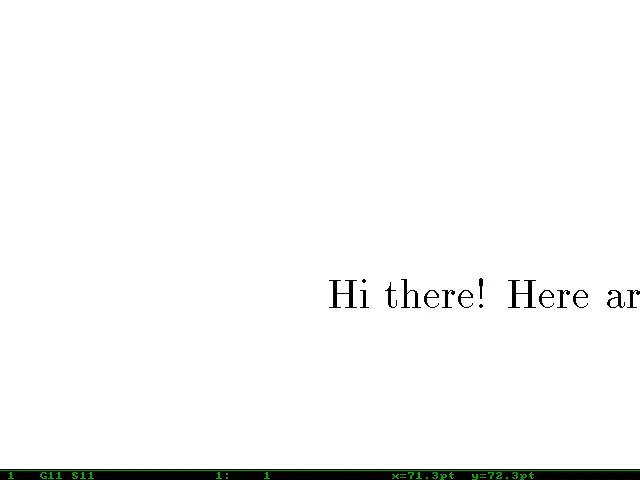

By default, V displays the document in a pretty close zoom, which is probably not what you want. You can use the + and - keys on your keyboard to adjust the zoom and the Up and Down arrow keys to move the “view window” up and down the page. If the document has more than one page, use the PgUp and PgDn keys to change to the next page. For example, here’s a view of the same document after zooming out a bit:

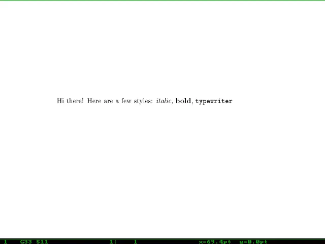
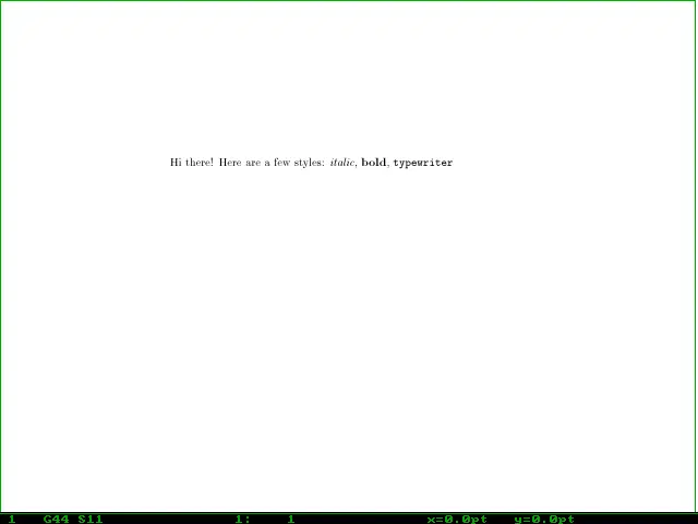
That green line indicates the page border; in this case, that’s the top of the page. If we zoom out just a little further with the - key, we can see the full width of the document:

A sample document with emTeX

As an undergraduate physics student, I used emTeX to write all of my lab reports. LaTeX makes it easy to format equations and other mathematics, which was very important to show the theory behind each experiment. For example, to format short math expressions in the body of a paragraph, you simply surround the statement with dollar signs, like $A = w \times h$ to indicate the area of a rectangle. For more intricate mathematics, you might instead format it as a block equation, using \begin{equation} and \end{equation}. LaTeX also supports other symbols using the backslash, like \times and \div to represent multiplication (×) and division (÷), and Greek letters such as \alpha (α) and \pi (π).

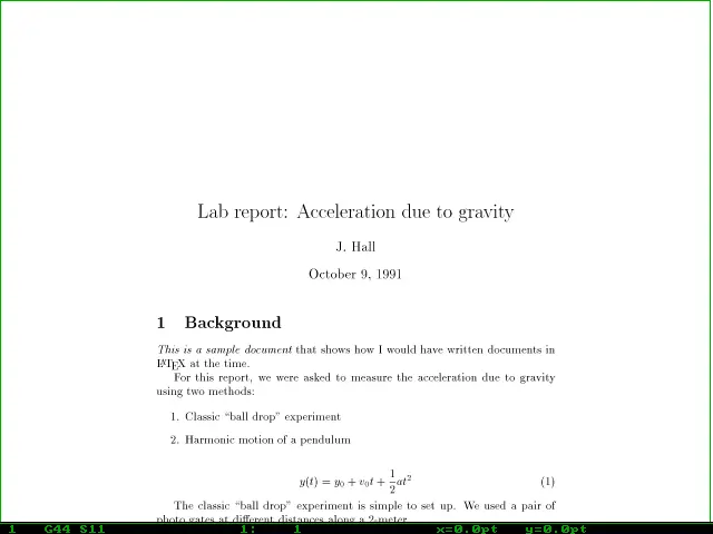
LaTeX also supports other formatting, including document titles, section and subsection headings, enumerated or “number” lists, and itemized or “bullet” lists. This formatting is necessary for nontrivial documents, such as this introduction to a lab report that I might have written as an undergraduate student using the “LaTeX 2.09” document style:

\documentstyle{article}
\begin{document}

\title{Lab report: Acceleration due to gravity}
\author{J. Hall}
\date{October 9, 1991}
\maketitle

\section{Background}

{\em This is a sample document} that shows how I would have written
documents in \LaTeX\ at the time.

For this report, we were asked to measure the acceleration due to
gravity using two methods:

\begin{enumerate}
 \item Classic ``ball drop'' experiment
 \item Harmonic motion of a pendulum
\end{enumerate}

\begin{equation}
y(t) = y_0 + v_0 t + \frac{1}{2} a t^2
\end{equation}

The classic ``ball drop'' experiment is simple to set up. We used a
pair of photo gates at different distances along a 2-meter ...

\end{document}

Let’s save this as labintro.tex and process it with emTeX. Again, emTeX complains about the old-style \documentstyle, so I’ve skipped much of the warning text with “…”

> latex2e labintro
...
 New documents should use Standard LaTeX conventions and start
 with the \documentclass command.

 Compatibility mode is UNLIKELY TO WORK with LaTeX 2.09 style
 files that change any internal macros, especially not with
 those that change the FONT SELECTION or OUTPUT ROUTINES.

 Therefore such style files MUST BE UPDATED to use
          Current Standard LaTeX: LaTeX2e.
 If you suspect that you may be using such a style file, which
 is probably very, very old by now, then you should attempt to
 get it updated by sending a copy of this error message to the
 author of that file.
 *************************************************************

(d:/apps/emtex/texinput/latex2e/tracefnt.sty)
(d:/apps/emtex/texinput/latex2e/latexsym.sty))
(d:/apps/emtex/texinput/latex2e/article.cls
Document Class: article 1998/05/05 v1.3y Standard LaTeX document class
(d:/apps/emtex/texinput/latex2e/size10.clo))
No file labintro.aux.
(d:/apps/emtex/texinput/latex2e/ulasy.fd) [1] (labintro.aux) )
Output written on labintro.dvi (1 page, 1348 bytes).
Transcript written on labintro.log.

This produces a labintro.dvi file that we can view with the V program. I’ve zoomed out the document in this screenshot to show only the top of the page; the document actually ends there anyway, so the rest of the page would be blank:

Writing with emTeX

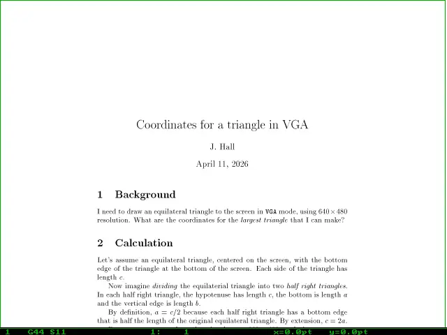
Now that we’ve seen how to write a few sample documents in LaTeX and how to process them and view the output using emTeX, let’s look at a more typical example, this time as a LaTeX2e document. LaTeX excels at formatting documents that include mathematics, so I’ll demonstrate by writing a short paper about how to calculate the coordinates of an equilateral triangle.

This document includes many features that technical writers might typically use in a LaTeX document, but it is the mathematics that make it stand out. Note that this uses both numbered and unnumbered equations, as well as inline mathematical expressions, and other formatting such as bold, italic, and typewriter styles.

The equations are noteworthy because they start out pretty simple but require more advanced formatting later on. Yet LaTeX makes it easy to write the equations using notation that’s fairly representative of how it should be printed:

\documentclass{article}
\begin{document}

\title{Coordinates for a triangle in VGA}
\author{J. Hall}
\date{\today}
\maketitle

\section{Background}

I need to draw an equilateral triangle to the screen
in \texttt{VGA} mode, using $640 \times 480$ resolution.
What are the coordinates for the \emph{largest triangle}
that I can make?

\section{Calculation}

Let's assume an equilateral triangle, centered on the
screen, with the bottom edge of the triangle at the
bottom of the screen. Each side of the triangle has
length $c$.

Now imagine \emph{dividing} the equilaterial triangle
into two \emph{half right triangles}.
In each half right triangle, the hypotenuse has length
$c$, the bottom is length $a$ and the vertical edge is
length $b$.

By definition, $a=c/2$ because each half right triangle
has a bottom edge that is half the length of the original
equilateral triangle. By extension, $c=2a$.

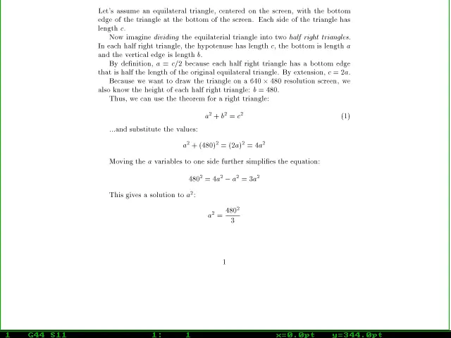
Because we want to draw the triangle on a $640 \times 480$
resolution screen, we also know the height of each half
right triangle: $b=480$.

Thus, we can use the theorem for a right triangle:

\begin{equation}
a^2 + b^2 = c^2
\end{equation}

...and substitute the values:

\begin{displaymath}
a^2 + (480)^2 = (2a)^2 = 4 a^2
\end{displaymath}

%% because 'displaymath' might be used frequently,
%% LaTeX also supports \[ and \] as a shorthand

Moving the $a$ variables to one side further simplifies
the equation:

\[
480^2 = 4 a^2 - a^2 = 3 a^2
\]

This gives a solution to $a^2$:

\[
a^2 = \frac{480^2}{3}
\]

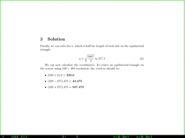
\section{Solution}

Finally, we can solve for $a$, which is half the length
of each side on the equilaterial triangle:

\begin{equation}
a = \sqrt{ \frac{480^2}{3} } \approx 277.1
\end{equation}

We can now calculate the coordinates.
To center an equilaterial triangle on the screen using
$640 \times 480$ resolution, the vertices should be:

\begin{itemize}
\item $(640 \div 2)$,$0$ = \textbf{320,0}
\item $(320-277)$,$479$ = \textbf{43,479}
\item $(320+277)$,$479$ = \textbf{597,479}
\end{itemize}

\end{document}

Let’s save this as vgatri.tex so we can process it using emTeX. This might be named more descriptively on a modern system like Windows, Mac, or Linux, but DOS systems could support only files with up to eight letters for the name and three letters for the extension. Some programs could support longer filenames with an extension, but the “8.3” filename limitation was well-known on DOS at the time, so I’ve used that here:

> latex2e vgatri
This is emTeX (tex386), Version 3.14159 [4b] (no format preloaded)
**&latex vgatri
(vgatri.tex
LaTeX2e <1998/06/01>
(d:/apps/emtex/texinput/latex2e/article.cls
Document Class: article 1998/05/05 v1.3y Standard LaTeX document class
(d:/apps/emtex/texinput/latex2e/size10.clo))
No file vgatri.aux.
[1] (d:/apps/emtex/texinput/latex2e/omscmr.fd) [2] (vgatri.aux) )
Output written on vgatri.dvi (2 pages, 3204 bytes).
Transcript written on vgatri.log.

This produces a two-page document, which we can view with V. You will need to use the Up and Down arrow keys to move the “view window” to see the full contents of the first page:

Use the PgDn key to view the second page of the document. The content on the second page is quite short, and shows up on one screen:

---

Thanks to Kate Lee for editing! Kate is a technical writer and editor in Minneapolis, Minnesota. She earned her BS in Technical Writing from the University of Minnesota in May 2026. Kate did an excellent job with copyediting and focusing the article.